在使用Pychem的过程中，如何导入数据以及分类

电脑 2023-03-15

python：怎么把文本中的这些数据导入到字典中再分类呢

1。数据--获取外部数据--自文本。我是excel 2010 。其他的版本也是在数据里面，差不多。 2。直接复制粘贴到excel ，然后在数据——分列

数据分析员用python做数据分析是怎么回事，需要用到python中的那些内容，具体是怎么操作的?

最近，Analysis with Programming加入了Planet Python。我这里来分享一下如何通过Python来开始数据分析。具体内容如下：

数据导入

导入本地的或者web端的CSV文件；

数据变换；

数据统计描述；

假设检验

单样本t检验；

可视化；

创建自定义函数。

数据导入

1
这是很关键的一步，为了后续的分析我们首先需要导入数据。通常来说，数据是CSV格式，就算不是，至少也可以转换成CSV格式。在Python中，我们的操作如下：
import pandas as pd
# Reading data locally
df = pd.read_csv('/Users/al-ahmadgaidasaad/Documents/d.csv')
# Reading data from web
data_url = "https://raw.githubusercontent.com/alstat/Analysis-with-Programming/master/2014/Python/Numerical-Descriptions-of-the-Data/data.csv"
df = pd.read_csv(data_url)
为了读取本地CSV文件，我们需要pandas这个数据分析库中的相应模块。其中的read_csv函数能够读取本地和web数据。
END

数据变换

1
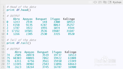
既然在工作空间有了数据，接下来就是数据变换。统计学家和科学家们通常会在这一步移除分析中的非必要数据。我们先看看数据（下图）
对R语言程序员来说，上述操作等价于通过print(head(df))来打印数据的前6行，以及通过print(tail(df))来打印数据的后6行。当然Python中，默认打印是5行，而R则是6行。因此R的代码head(df, n = 10)，在Python中就是df.head(n = 10)，打印数据尾部也是同样道理
请点击输入图片描述
2
在R语言中，数据列和行的名字通过colnames和rownames来分别进行提取。在Python中，我们则使用columns和index属性来提取，如下：
# Extracting column names
print df.columns
# OUTPUT
Index([u'Abra', u'Apayao', u'Benguet', u'Ifugao', u'Kalinga'], dtype='object')
# Extracting row names or the index
print df.index
# OUTPUT
Int64Index([0, 1, 2, 3, 4, 5, 6, 7, 8, 9, 10, 11, 12, 13, 14, 15, 16, 17, 18, 19, 20, 21, 22, 23, 24, 25, 26, 27, 28, 29, 30, 31, 32, 33, 34, 35, 36, 37, 38, 39, 40, 41, 42, 43, 44, 45, 46, 47, 48, 49, 50, 51, 52, 53, 54, 55, 56, 57, 58, 59, 60, 61, 62, 63, 64, 65, 66, 67, 68, 69, 70, 71, 72, 73, 74, 75, 76, 77, 78], dtype='int64')
3
数据转置使用T方法，
# Transpose data
print df.T
# OUTPUT
0 1 2 3 4 5 6 7 8 9
Abra 1243 4158 1787 17152 1266 5576 927 21540 1039 5424
Apayao 2934 9235 1922 14501 2385 7452 1099 17038 1382 10588
Benguet 148 4287 1955 3536 2530 771 2796 2463 2592 1064
Ifugao 3300 8063 1074 19607 3315 13134 5134 14226 6842 13828
Kalinga 10553 35257 4544 31687 8520 28252 3106 36238 4973 40140
... 69 70 71 72 73 74 75 76 77
Abra ... 12763 2470 59094 6209 13316 2505 60303 6311 13345
Apayao ... 37625 19532 35126 6335 38613 20878 40065 6756 38902
Benguet ... 2354 4045 5987 3530 2585 3519 7062 3561 2583
Ifugao ... 9838 17125 18940 15560 7746 19737 19422 15910 11096
Kalinga ... 65782 15279 52437 24385 66148 16513 61808 23349 68663
78
Abra 2623
Apayao 18264
Benguet 3745
Ifugao 16787
Kalinga 16900
Other transformations such as sort can be done using sort attribute. Now let's extract a specific column. In Python, we do it using either iloc or ix attributes, but ix is more robust and thus I prefer it. Assuming we want the head of the first column of the data, we have
4
其他变换，例如排序就是用sort属性。现在我们提取特定的某列数据。Python中，可以使用iloc或者ix属性。但是我更喜欢用ix，因为它更稳定一些。假设我们需数据第一列的前5行，我们有：
print df.ix[:, 0].head()
# OUTPUT 0 1243 1 4158 2 1787 3 17152 4 1266 Name: Abra, dtype: int64
5
顺便提一下，Python的索引是从0开始而非1。为了取出从11到20行的前3列数据，我们有
print df.ix[10:20, 0:3]
# OUTPUT
Abra Apayao Benguet
10 981 1311 2560
11 27366 15093 3039
12 1100 1701 2382
13 7212 11001 1088
14 1048 1427 2847
15 25679 15661 2942
16 1055 2191 2119
17 5437 6461 734
18 1029 1183 2302
19 23710 12222 2598
20 1091 2343 2654
上述命令相当于df.ix[10:20, ['Abra', 'Apayao', 'Benguet']]。
6
为了舍弃数据中的列，这里是列1(Apayao)和列2(Benguet)，我们使用drop属性，如下：
print df.drop(df.columns[[1, 2]], axis = 1).head()
# OUTPUT
Abra Ifugao Kalinga
0 1243 3300 10553
1 4158 8063 35257
2 1787 1074 4544
3 17152 19607 31687
4 1266 3315 8520
axis参数告诉函数到底舍弃列还是行。如果axis等于0，那么就舍弃行。
END

统计描述

1
下一步就是通过describe属性，对数据的统计特性进行描述：
print df.describe()
# OUTPUT
Abra Apayao Benguet Ifugao Kalinga
count 79.000000 79.000000 79.000000 79.000000 79.000000
mean 12874.379747 16860.645570 3237.392405 12414.620253 30446.417722
std 16746.466945 15448.153794 1588.536429 5034.282019 22245.707692
min 927.000000 401.000000 148.000000 1074.000000 2346.000000
25% 1524.000000 3435.500000 2328.000000 8205.000000 8601.500000
50% 5790.000000 10588.000000 3202.000000 13044.000000 24494.000000
75% 13330.500000 33289.000000 3918.500000 16099.500000 52510.500000
max 60303.000000 54625.000000 8813.000000 21031.000000 68663.000000
END

假设检验

1
Python有一个很好的统计推断包。那就是scipy里面的stats。ttest_1samp实现了单样本t检验。因此，如果我们想检验数据Abra列的稻谷产量均值，通过零假设，这里我们假定总体稻谷产量均值为15000，我们有：
from scipy import stats as ss
# Perform one sample t-test using 1500 as the true mean
print ss.ttest_1samp(a = df.ix[:, 'Abra'], popmean = 15000)
# OUTPUT
(-1.1281738488299586, 0.26270472069109496)
返回下述值组成的元祖：
t : 浮点或数组类型t统计量
prob : 浮点或数组类型two-tailed p-value 双侧概率值
2
通过上面的输出，看到p值是0.267远大于α等于0.05，因此没有充分的证据说平均稻谷产量不是150000。将这个检验应用到所有的变量，同样假设均值为15000，我们有：
print ss.ttest_1samp(a = df, popmean = 15000)
# OUTPUT
(array([ -1.12817385, 1.07053437, -65.81425599, -4.564575 , 6.17156198]),
array([ 2.62704721e-01, 2.87680340e-01, 4.15643528e-70,
1.83764399e-05, 2.82461897e-08]))
第一个数组是t统计量，第二个数组则是相应的p值
END

可视化

1
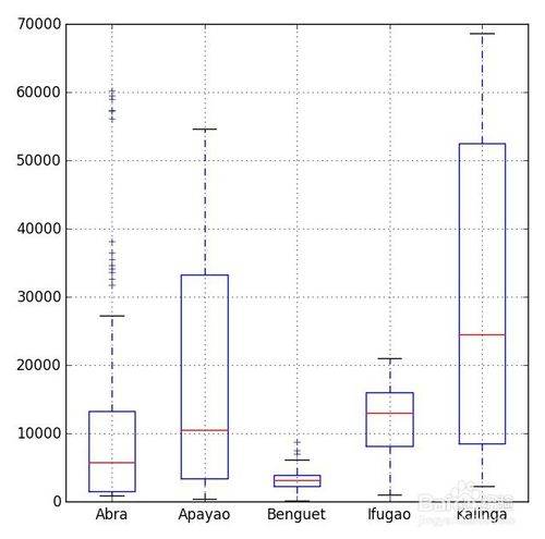
Python中有许多可视化模块，最流行的当属matpalotlib库。稍加提及，我们也可选择bokeh和seaborn模块。之前的博文中，我已经说明了matplotlib库中的盒须图模块功能。
请点击输入图片描述
2
# Import the module for plotting
import matplotlib.pyplot as plt
plt.show(df.plot(kind = 'box'))
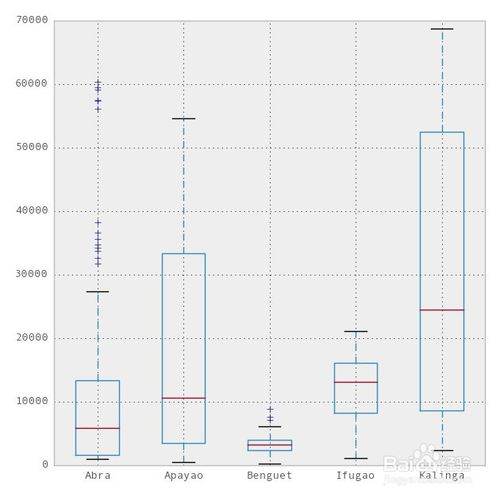
现在，我们可以用pandas模块中集成R的ggplot主题来美化图表。要使用ggplot，我们只需要在上述代码中多加一行，
import matplotlib.pyplot as plt
pd.options.display.mpl_style = 'default' # Sets the plotting display theme to ggplot2
df.plot(kind = 'box')
3
这样我们就得到如下图表：
请点击输入图片描述
4
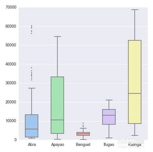
比matplotlib.pyplot主题简洁太多。但是在本文中，我更愿意引入seaborn模块，该模块是一个统计数据可视化库。因此我们有：
# Import the seaborn library
import seaborn as sns
# Do the boxplot
plt.show(sns.boxplot(df, widths = 0.5, color = "pastel"))
请点击输入图片描述
5
多性感的盒式图，继续往下看。
请点击输入图片描述
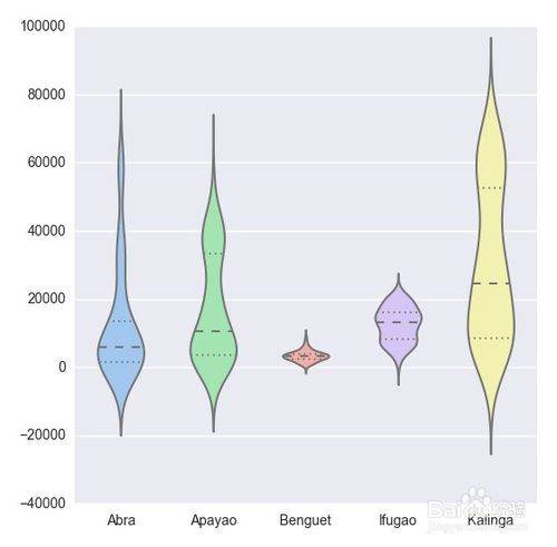
6
plt.show(sns.violinplot(df, widths = 0.5, color = "pastel"))
请点击输入图片描述
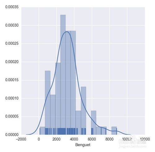
7
plt.show(sns.distplot(df.ix[:,2], rug = True, bins = 15))
请点击输入图片描述
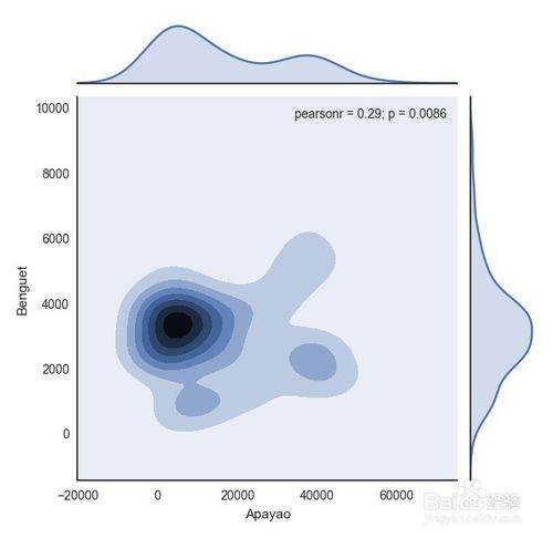
8
with sns.axes_style("white"):
plt.show(sns.jointplot(df.ix[:,1], df.ix[:,2], kind = "kde"))
请点击输入图片描述
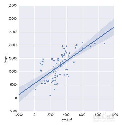
9
plt.show(sns.lmplot("Benguet", "Ifugao", df))
END

创建自定义函数

在Python中，我们使用def函数来实现一个自定义函数。例如，如果我们要定义一个两数相加的函数，如下即可：
def add_2int(x, y):
return x + y
print add_2int(2, 2)
# OUTPUT
4
顺便说一下，Python中的缩进是很重要的。通过缩进来定义函数作用域，就像在R语言中使用大括号{…}一样。这有一个我们之前博文的例子：
产生10个正态分布样本，其中和
基于95%的置信度，计算和;
重复100次; 然后
计算出置信区间包含真实均值的百分比
Python中，程序如下：
import numpy as np
import scipy.stats as ss
def case(n = 10, mu = 3, sigma = np.sqrt(5), p = 0.025, rep = 100):
m = np.zeros((rep, 4))
for i in range(rep):
norm = np.random.normal(loc = mu, scale = sigma, size = n)
xbar = np.mean(norm)
low = xbar - ss.norm.ppf(q = 1 - p) * (sigma / np.sqrt(n))
up = xbar + ss.norm.ppf(q = 1 - p) * (sigma / np.sqrt(n))
if (mu > low) & (mu < up):
rem = 1
else:
rem = 0
m[i, :] = [xbar, low, up, rem]
inside = np.sum(m[:, 3])
per = inside / rep
desc = "There are " + str(inside) + " confidence intervals that contain "
"the true mean (" + str(mu) + "), that is " + str(per) + " percent of the total CIs"
return {"Matrix": m, "Decision": desc}
上述代码读起来很简单，但是循环的时候就很慢了。下面针对上述代码进行了改进，这多亏了Python专家
import numpy as np
import scipy.stats as ss
def case2(n = 10, mu = 3, sigma = np.sqrt(5), p = 0.025, rep = 100):
scaled_crit = ss.norm.ppf(q = 1 - p) * (sigma / np.sqrt(n))
norm = np.random.normal(loc = mu, scale = sigma, size = (rep, n))
xbar = norm.mean(1)
low = xbar - scaled_crit
up = xbar + scaled_crit
rem = (mu > low) & (mu < up)
m = np.c_[xbar, low, up, rem]
inside = np.sum(m[:, 3])
per = inside / rep
desc = "There are " + str(inside) + " confidence intervals that contain "
"the true mean (" + str(mu) + "), that is " + str(per) + " percent of the total CIs"
return {"Matrix": m, "Decision": desc}

如何在python中进行数据库的添加

你可以访问Python数据库接口及API查看详细的支持数据库列表。不同的数据库你需要下载不同的DB API模块，例如你需要访问Oracle数据库和Mysql数据，你需要下载Oracle和MySQL数据库模块。 DB-API 是一个规范. 它定义了一系列必须的对象和数据库存取方式, 以便为各种各样的底层数据库系统和多种多样的数据库接口程序提供一致的访问接口。 Python的DB-API，为大多数的数据库实现了接口，使用它连接各数据库后，就可以用相同的方式操作各数据库。 Python DB-API使用流程：引入 API 模块。获取与数据库的连接。执行SQL语句和存储过程。关闭数据库连接。

怎么把chemdraw里的分子导入到pymol里

ChemDraw中画出的分子结构，直接复制粘贴到Chem3D中即可。然后生成3维图形。ChemDraw面板可以绘制二维结构式，所以一般无需再拷贝到ChemDraw中，拷贝可以的，还是直接复制粘贴。

如何在商品列表中增加新商品，并导入数据？

在开始使用本工具前，需要做初期的一些简单配置。第一，配置飞狐目录下的Config.ini文件修改=C:\Program Files\CES MT4\history\Aksys-Demo\为你当前使用中的MT4对应历史数据文件夹。然后保存。第二，成功登陆飞狐系统后，进入任意商品的图形界面（K线图），添加技术指标 MT4 STOCK 位于工具栏RSI--技术指标--其它--MT4 STOCK第三，加载指标成功后，滚动商品检查飞狐接收数据是否一切正常。逐次点击1分钟，5分钟，15分钟，30分钟， 60分钟，240分钟，日图，周图，使其自动生成数据文件后，并将窗口大小调整至适当大小，放置桌面底部。防

标签：信息技术编程语言 python 数据分析商品列表